Temporal Convolution Networks
What is a Temporal Convolution Network? What are its building blocks? A working implementation using fast.ai and tsai


- Objective
- sequence modelling had become synonymous with recurrent networks.
- This paper shows that convolutional networks can outperform recurrent networks on some of the tasks.
- paper concludes that common association between sequence modelling and recurrent networks should be reconsidered.
- A new general architecture for convolutional sequence prediction.
- This new general architecture is referred to as
Temporal Convolutional Networksabbreviated asTCN. - Convolutions in this architecture are
causalwhich means that there is no information leakage. - Architecture can take in a sequence of arbitrary length and map it to an output sequence of the same length, just like RNNs. ( But
tcnachieves this function not throughseq2seqbut simply usingconvolutionallayers. ) - Also this paper highlights how we could combine deep networks ( with residual structures ) and dilated convolutions could be used to build long term dependencies. ( ability of an model to look back in past to make future predictions )
What is a sequence modelling task?
Taken directly from paper
Before defining the network structure, we highlight the nature of the sequence modeling task. Suppose that we are given an input sequence $x_0$, . . . , $x_T$ , and wish to predict some corresponding outputs $y_0$, . . . , $y_T$ at each time. The key constraint is that to predict the output $y_t$ for some time t, we are constrained to only use those inputs that have been previously observed:$x_0$, . . . , $x_t$. Formally, a sequence modeling network is any function f : $X_{T +1}$ → $Y_{T +1}$ that produces the mapping
$y_0$, . . . , $y_T$ = f($x_0$, . . . , $x_T$ ) (1)
if it satisfies the causal constraint that $y_t$ depends only on $x_0$, . . . , $x_t$ and not on any “future” inputs $x_{t+1}$, . . . , $x_T$. The goal of learning in the sequence modeling setting is to find a network f that minimizes some expected loss between the actual outputs and the predictions.
L($y_0$, . . . , $y_T$ , f($x_0$, . . . , $x_T$)), where the sequences and outputs are drawn according to some distribution.
What is a 1D convolution?
Before we jump into the paper we must understand what is a 1D convolution since it is used in the causal convolutional layer in TCN
- 1D Convolution takes in a 3D tensor as input and outputs a 3D tensor as output.
- Shape of the input tensor in
TCNwould have following dimension ( batch_size, input_length, input_size ) and the output tensor has shape ( batch_size, input_length, output_size ) - Each layer in
TCNhas same input and output length so only the third dimension would change.
In the above figure we can notice the follwing
- to compute a single output we need to look at 3 consecutive values of the input sequence, it is because we are using a kernel of size
3here. - to maintain that input and output sequences be of the same size we have to pad the input sequence with zeros on both sides.
- 1d convolution is a special case of 2d convolution
How is 1d convolution a special case of 2d convolution?
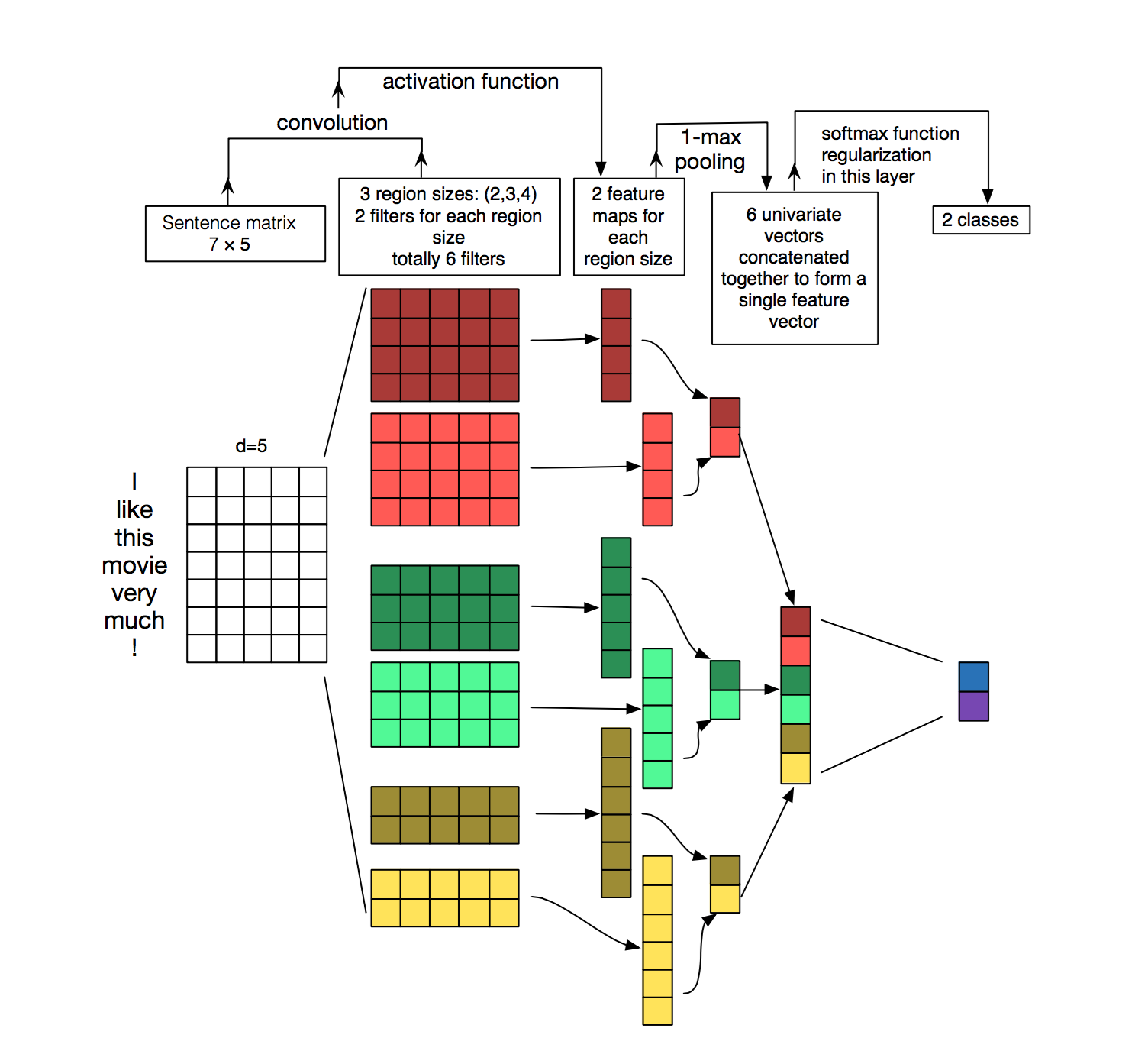
In both time series and NLP, data is laid out in a similar manner, in the figure above we have embedded the words I like this movie very much ! into a 7 x 5 embedding matrix and then we use 1d convolution on this 2D matrix.
1d convolution is a special case of 2d convolution where kernel size of the 1d convolution is it's height. The width of the kernel is defined by the embedding size, which is 5 here and it is fixed. So it means that we can only slide vertically and not horizontally which makes it 1D convolution.
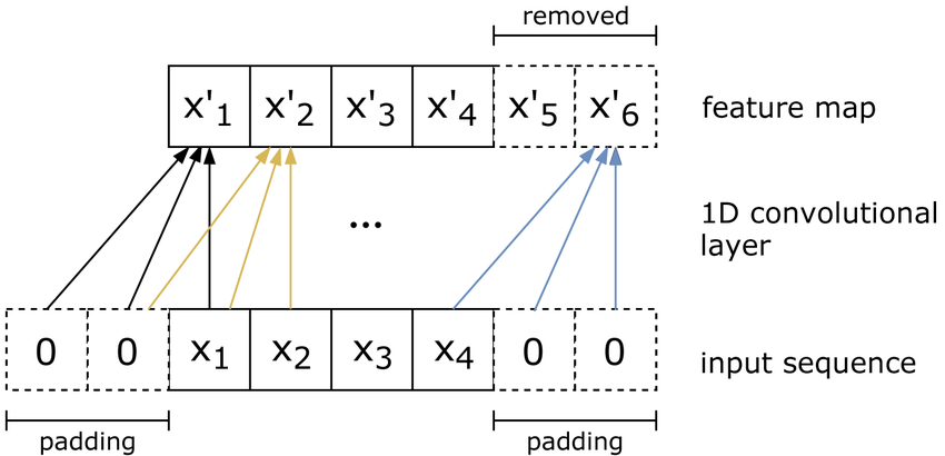
- Causality means that an element in the output sequence can only depend on elements that precede it in the input sequence.
- In order to ensure that an output tensor has the same length as the input tensor, we need to do zero padding.
- If we only pad the left side of the input tensor with zeros, then causal convolution is guaranteed.
- $x^{'}_4$ in the figure below is generated by combining $x_2$, $x_3$, $x_4$ which ensures no leakage of information.
This operation generates $x^{'}_5$ and $x^{'}_6$ which are extraneous and should be removed before passing the output to the next layer. We have to take care of it in the implementation.
How many zeros would be required to make sure that the output would be of same length as input?
(kernel_size - 1)
TCN has two basic principles:
- input and output length of the sequences remain same.
- there can be no leakage from the past.
To achieve the first point TCN makes use of 1D FCN ( Fully Convolutional Network ) and to achieve the second point TCN makes use of causal convolutions.
Disadvantages of the above architecture
- To model long term dependencies, we need a very deep network or very large convolution kernels, neither of which turned out to be particularly feasible in the experiments.
-
A desirable quality of a the model is that the value of a particular entry in the output depends on all previous entries in the input.
-
This is achieved when the size of the receptive field is equal to the length of the input.
-
We could expand our receptive field when we stack multiple layers together. In the figure below we can see that by stacking two layers with kernel_size 3, we get a receptive field size of 5.

In general, the receptive field r of a 1D convolutional network with n layers and kernel_size k is
$r = 1 + n * ( k - 1 )$
To know how many layers are needed for full coverage, we can set the receptive field size to input_length l and solve for the number of layers n (non-integer values need to be rounded):
$\lceil\frac{(l-1)}{(k-1)}\rceil$
This means that, with a fixed kernel_size, the number of layers required for complete coverage would be linear in input length. This will cause the network to become very deep and very fast, resulting in models with a large number of parameters that take longer to train.
How could we solve this issue?
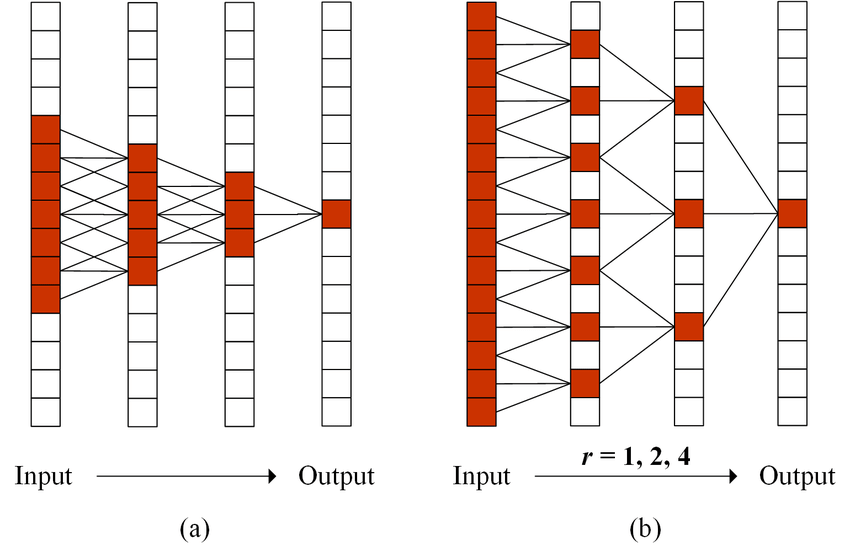
One way to increase the size of the receptive field while keeping the number of layers relatively small is to introduce the concept of dilation.
Dilation in the context of convolutional layers refers to the distance between elements of the input sequence that are used to compute one entry of the output sequence. Therefore, a traditional convolutional layer can be viewed as a layer dilated by 1, because the input elements involved in calculating output value are adjacent.
The image below shows an example of how the receptive field grows when we introduce dilation. The right side image uses a dilation rate r 1 in the first layer with kernel_size 3 which is how a traditional conv layer would work although in the next layer we use r=2 which makes sure that we combine input elements that are 2 elements apart when producing output for the next layer and so on.
To overcome the problem of number of layers required for covering the entire input length we must progressively increase the dilation rate over multiple layers.
This problem can be solved by exponentially increasing the value of d as we move up in the layer. To do this, we choose a constant dilation_base integer b that will allow us to calculate the dilation d for a particular layer based on the number of layers i under it, i.e. $d = b^i$.
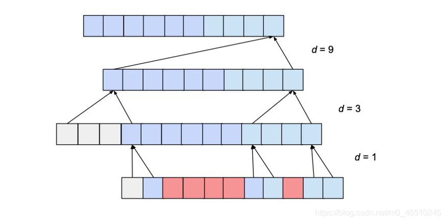
The figure below shows a network with an input_length of 10, a kernel_size of 3, and a dilation_base of 2, which would result in a complete coverage of the 3 dilated convolutional layers.
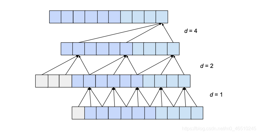
Here we can see that the all input values are used to produce the last value in the output layer. With the above mentioned setup we could have an input of length 15 while maintaining the full coverage.
How did we calculate that the receptive width is 15?
- When a layer is added to the architecture the receptive field is increased by $d*(k-1)$
- So if we have n layers with kernel_size k and dilation base rate as b then receptive width is calculated as
$w=1+(k-1)\frac{b^n-1}{b-1}$
but depending on values of b and k the architecture could have many holes in it.
What does that mean?
Here we can see not all inputs are used to compute the last value of the output, even though w is greater than the input size. To fix this we would have to either increase the kernel size or decrease the dilation rate from 3 to 2. In general we must ensure that kernel_size is atleast equal to dilation rate to avoid such cases.
How many layers would be required for full coverage?
Given a kernel size k, a dilation base b where k ≥ b, and an input length l, in order to achieve full coverage following condition must be satisfied
$1+(k-1)\frac{b^n-1}{b-1}\geq l$, then
$n=\lceil\log_b(\frac{(l-1)*(b-1)}{k-1}+1)\rceil$
Now number of layers is lograthmic in input layer length l which is what we wanted. This is a significant improvement that can be achieved without sacrificing receptive field coverage.
Now, the only thing that needs to be specified is the number of zero-padded items required for each layer. Assuming that the dilation expansion base is b, the kernel size is k, and there are i layers below the current layer, the number p of zero-padding items required by the current layer is calculated as follows:
$p=b^i*(k-1)$
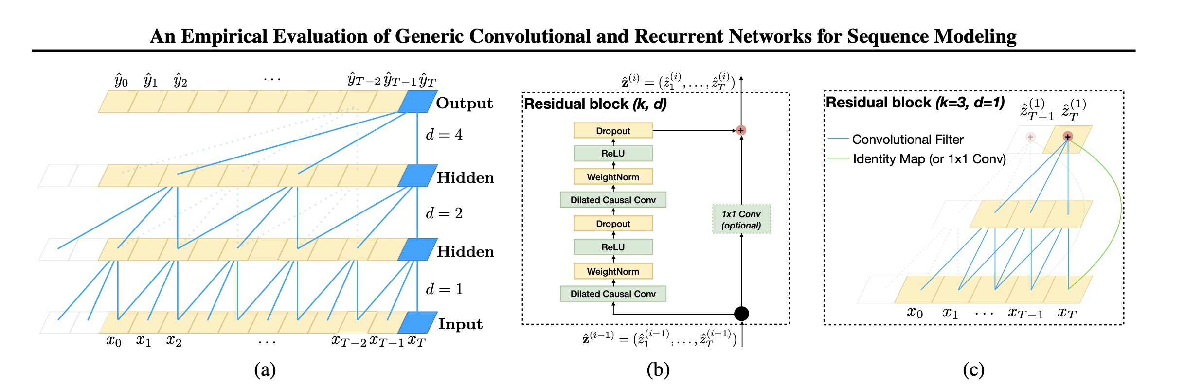
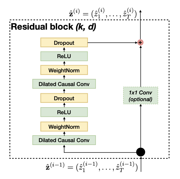
- Residual links have proven to be an effective way to train deep networks, which allow the network to pass information in a cross-layer manner.
- This paper constructs a residual block to replace one layer of convolution. As shown in the figure above, a residual block contains two layers of convolution and nonlinear mapping, and WeightNorm and Dropout are added to each layer to regularize the network.
-
Each hidden layer has the same length as the input layer, and is padded with zeros to ensure subsequent layers have the same length.
-
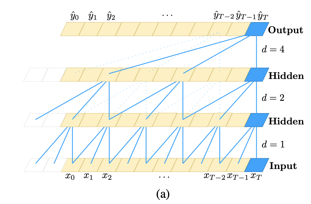
For the output at time t, the causal convolution (convolution with causal constraints) uses the input at time t and the previous layer at an earlier time (see the blue line connection at the bottom of the figure above).
-
Causal convolution is not a new idea, but the paper incorporates very deep networks to allow for long-term efficient histories.
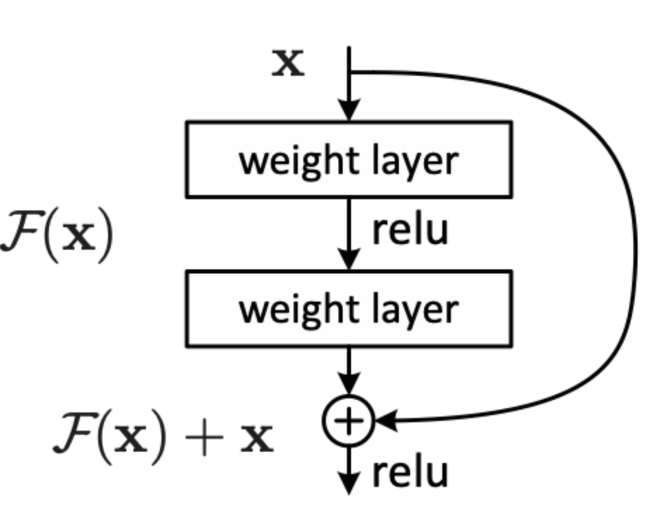
- Residual blocks (originally from ResNet) have repeatedly shown to benefit very deep networks.
- Since the receptive field of a TCN depends on the network depth
nas well as the convolution kernel sizekand dilation factord, it becomes very important to stabilize deeper and larger TCNs. - Predictions may depend on long historical values and high-dimensional input sequences. e.g An input sequence of size $2^{12}$ may require a network of up to 12 layers.
- In standard ResNet, the input is directly added to the output of the residual function, while in TCN the input and output can have different widths. To account for the difference in input-output width, an additional
1x1convolution is used to ensure that element-wise addition receives tensors of the same shape.
- The innovation in the TCN model is to sort out how to use causal and dilated convolutions to solve the sequence modelling task.
- Causal and Dilated convolutions have already been proposed earlier but this paper highlights how they could be combined together for sequence modelling tasks
Advantages
-
Parallelism. When given a sentence, TCN can process the sentence in parallel without the need for sequential processing like RNN.
-
Flexible receptive field. The size of the receptive field of TCN is determined by the number of layers, the size of the convolution kernel, and the expansion coefficient. It can be flexibly customized according to different characteristics of different tasks.
-
Stable gradient. RNN often has the problems of vanishing gradients and gradient explosion, which are mainly caused by sharing parameters in different time periods. Like traditional convolutional neural networks, TCN does not have the problem of gradient disappearance and explosion.
-
Lower memory requirements. When RNN is used, it needs to save the information of each step, which will occupy a lot of memory. The convolution kernel of TCN is shared in one layer, and hence lower memory usage.
Disadvantages
-
TCN may not be so adaptable in transfer learning. This is because the amount of historical information required for model predictions may be different in different domains. Therefore, when migrating a model from a problem that requires less memory information to a problem that requires longer memory, TCN may perform poorly because its receptive field is not large enough.
-
The TCN described in the paper is also a one-way structure. In tasks such as speech recognition and speech synthesis, the pure one-way structure is quite useful. However, most of the texts use a bidirectional structure. Of course, it is easy to expand the TCN into a bidirectional structure. Instead of using causal convolution, the traditional convolution structure can be used.
-
TCN is a variant of convolutional neural network after all. Although the receptive field can be expanded by using dilated convolution, it is still limited. Compared with Transformer, it is still poor in capturing relevant information of any length. The application of TCN to text remains to be tested.
Tips for implementation
Next we would highlight things to keep in mind if you plan to implement the paper
- After the convolution, the size of the output data after the convolution is greater than the size of the input data
- This is caused owing to padding both sides, so we chomp off extra padded 0s from right side to get the desired data values.
We have taken this (https://github.com/locuslab/TCN/blob/2221de3323/TCN/tcn.py) implementation of TCN and implemented in fast.ai and tsai to demonstrate how TCN could be used for sequence modelling.
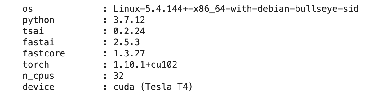
from tsai.all import *
computer_setup()
We are going to select appliances energy dataset recently released by Monash, UEA & UCR Time Series Extrinsic Regression Repository (2020)
dsid = 'AppliancesEnergy'
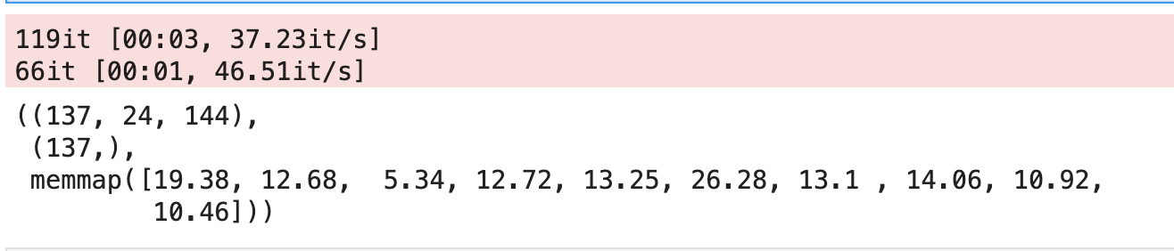
X, y, splits = get_regression_data(dsid, split_data=False)
X.shape, y.shape, y[:10]
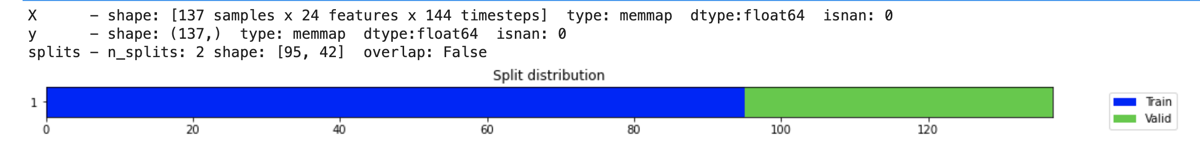
check_data(X, y, splits)
tfms  = [None, [TSRegression()]]
batch_tfms = TSStandardize(by_sample=True, by_var=True)
dls = get_ts_dls(X, y, splits=splits, tfms=tfms, batch_tfms=batch_tfms, bs=128)
dls.one_batch()
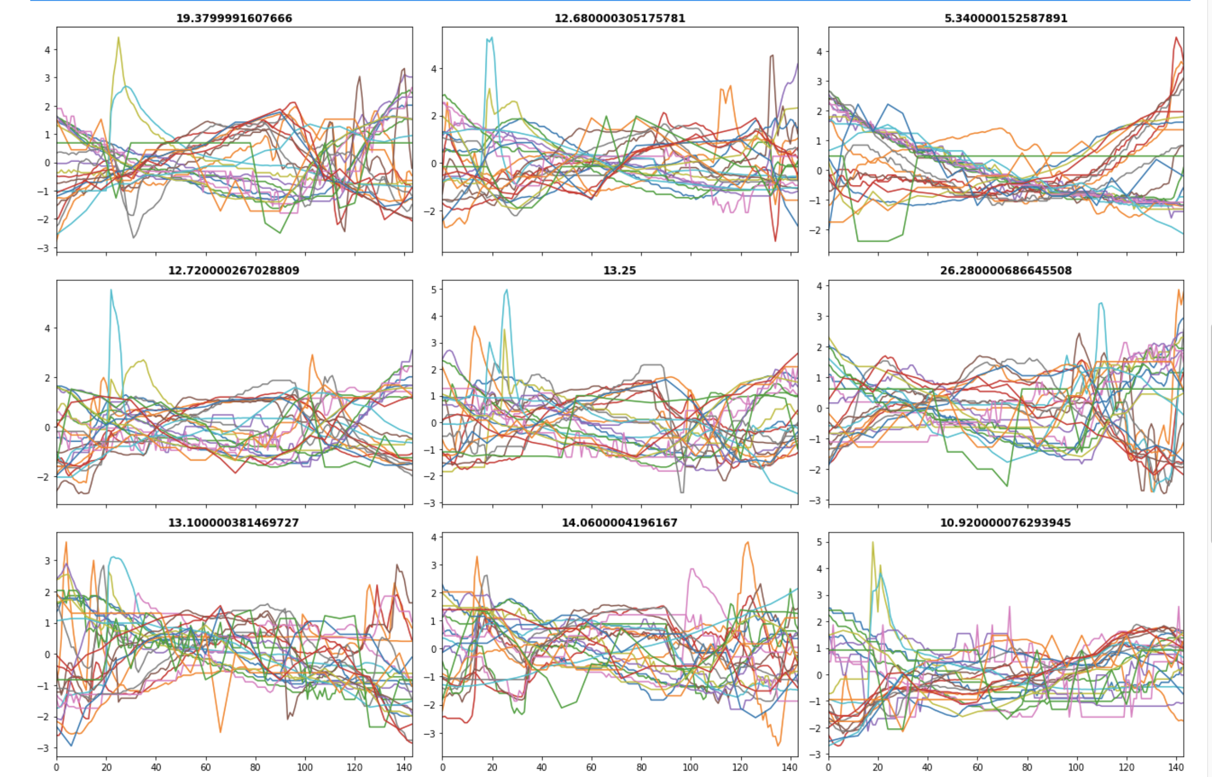
dls.show_batch()
from fastai.torch_basics import *
from fastai.tabular.core import *

from torch.nn.utils import weight_norm
class Chomp1d(Module):
    def __init__(self, chomp_size):
        store_attr()

    def forward(self, x):
        return x[:, :, :-self.chomp_size].contiguous()


def get_conv_block(n_inputs, n_outputs, kernel_size, stride, padding, dilation, dropout):
    conv  = weight_norm(nn.Conv1d(n_inputs,
                                  n_outputs,
                                  kernel_size,
                                  stride=stride,
                                  padding=padding,
                                  dilation=dilation
                                  ))
    chomp = Chomp1d(padding)
    relu  = nn.ReLU()
    drop  = nn.Dropout(dropout)

    return nn.Sequential(*(conv, chomp,
                           relu, drop
                        ))

class TemporalBlock(Module):
    def __init__(self, n_inputs, n_outputs, kernel_size, stride, dilation, padding, dropout=0.5):
        store_attr()

        self.in_conv_blk = get_conv_block(n_inputs,
                                          n_outputs,
                                          kernel_size,
                                          stride,
                                          padding,
                                          dilation,
                                          dropout
                                         )

        self.out_conv_blk = get_conv_block(n_outputs,
                                           n_outputs,
                                           kernel_size,
                                           stride,
                                           padding,
                                           dilation,
                                           dropout
                                          )

        self.net             = nn.Sequential(*(self.in_conv_blk, self.out_conv_blk))
        self.downsample_conv = nn.Conv1d(n_inputs, n_outputs, kernel_size=1) if n_inputs != n_outputs else None
        self.relu            = nn.ReLU()
        self.init_weights()

    def init_weights(self):
        # 0 index represents the convolutional layer
        self.in_conv_blk[0].weight.data.normal_(0, 0.01)
        self.out_conv_blk[0].weight.data.normal_(0, 0.01)
        if self.downsample_conv is not None:
            self.downsample_conv.weight.data.normal_(0, 0.01)

    def forward(self, x):
        out = self.net(x)
        res = x if self.downsample_conv is None else self.downsample_conv(x)
        return self.relu(out + res)

class TemporalConvNet(Module):
    def __init__(self, num_inputs, num_channels, kernel_size=2, dropout=0.2):
        layers     = []
        num_levels = len(num_channels)

        for i in range(num_levels):
            dilation_size = 2 ** i
            in_channels   = num_inputs if i == 0 else num_channels[i-1]
            out_channels  = num_channels[i]

            layers       += [TemporalBlock(in_channels,
                                           out_channels,
                                           kernel_size,
                                           stride=1,
                                           dilation=dilation_size,
                                           padding=(kernel_size-1) * dilation_size,
                                           dropout=dropout
                                          )
                            ]

        self.network = nn.Sequential(*layers)

    def forward(self, x):
        return self.network(x)

class TCN(Module):
    def __init__(self, input_size, output_size, num_channels, kernel_size, dropout):
        self.tcn    = TemporalConvNet(input_size, num_channels, kernel_size=kernel_size, dropout=dropout)
        self.linear = nn.Linear(num_channels[-1], output_size)
        self.init_weights()

    def init_weights(self):
        self.linear.weight.data.normal_(0, 0.01)

    def forward(self, x):
        y1 = self.tcn(x)
        return self.linear(y1[:, :, -1])
model = TCN(input_size=24,
output_size=1,
num_channels=[24, 32, 64],
kernel_size=2,
dropout=0.2
)
learn = Learner(dls, model, metrics=[mae, rmse], cbs=ShowGraph())
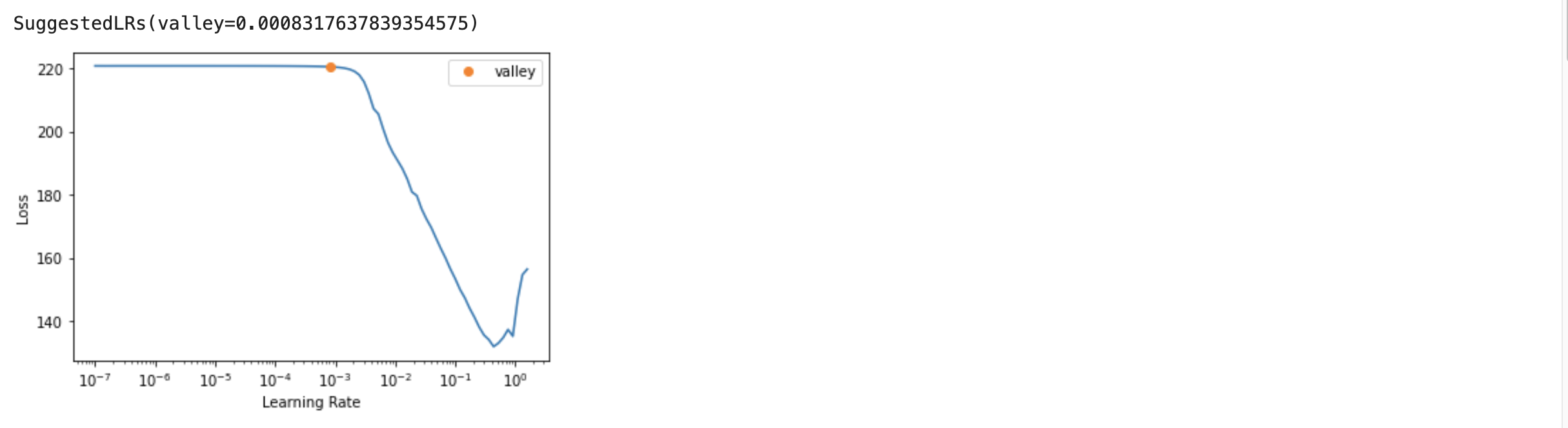
learn.lr_find()
model = TCN(input_size=24,
output_size=1,
num_channels=[24, 32, 64],
kernel_size=2,
dropout=0.2
)
learn = Learner(dls, model, metrics=[mae, rmse], cbs=ShowGraph())
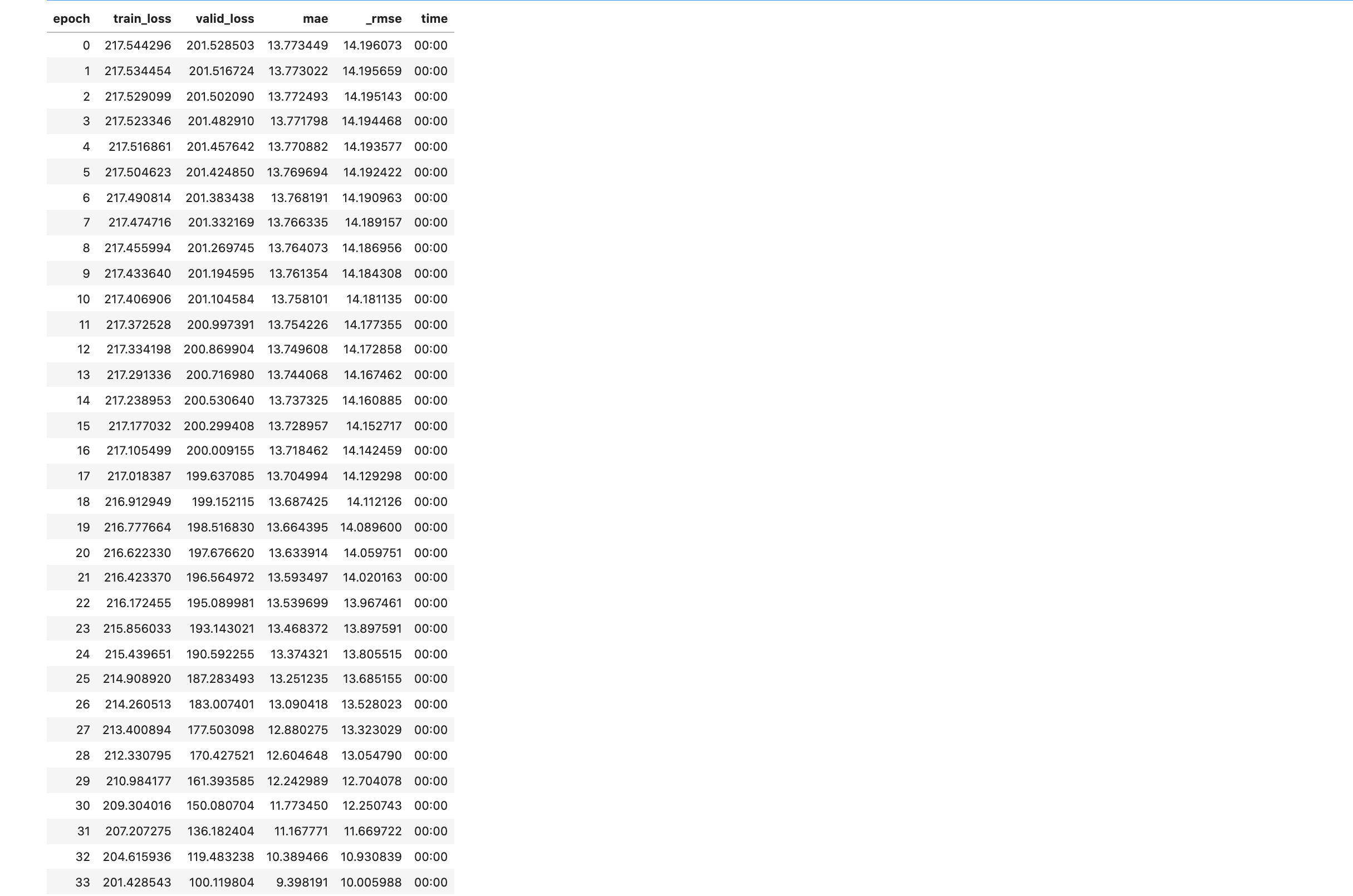
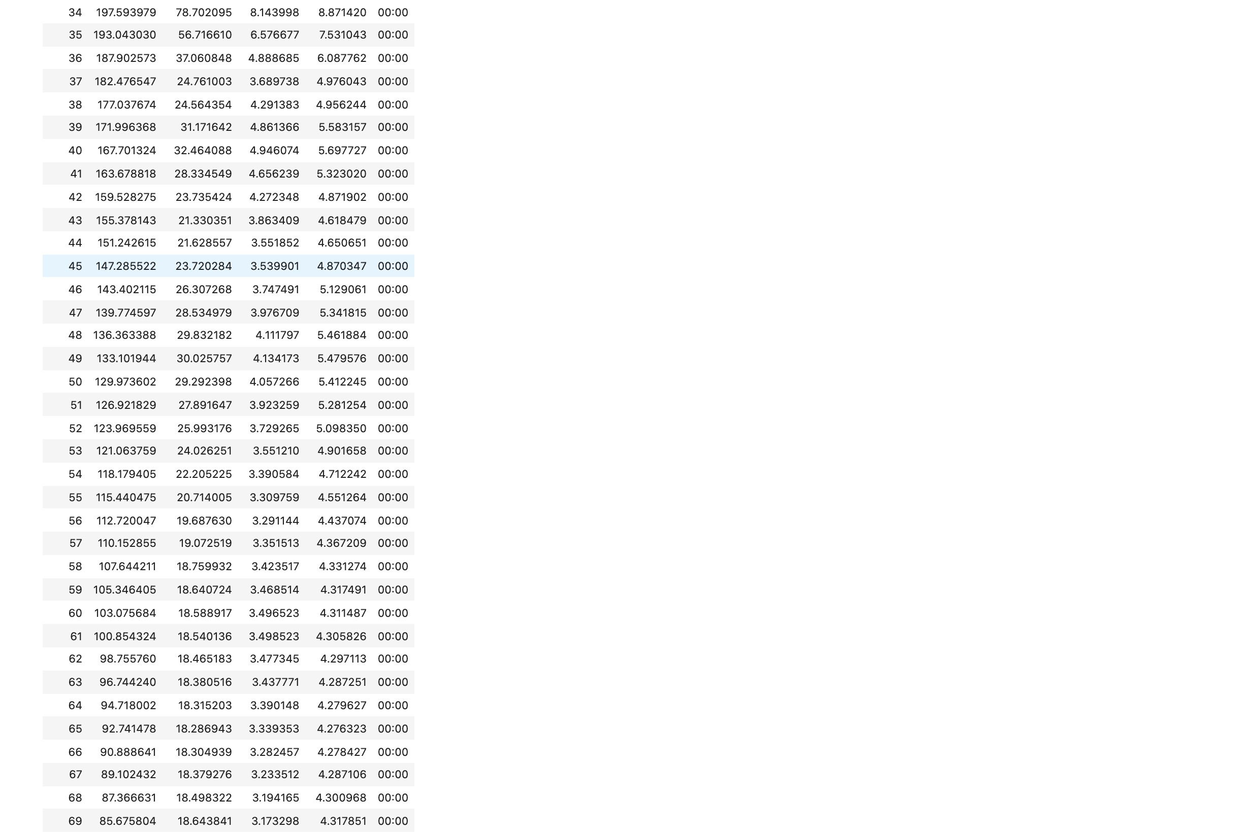
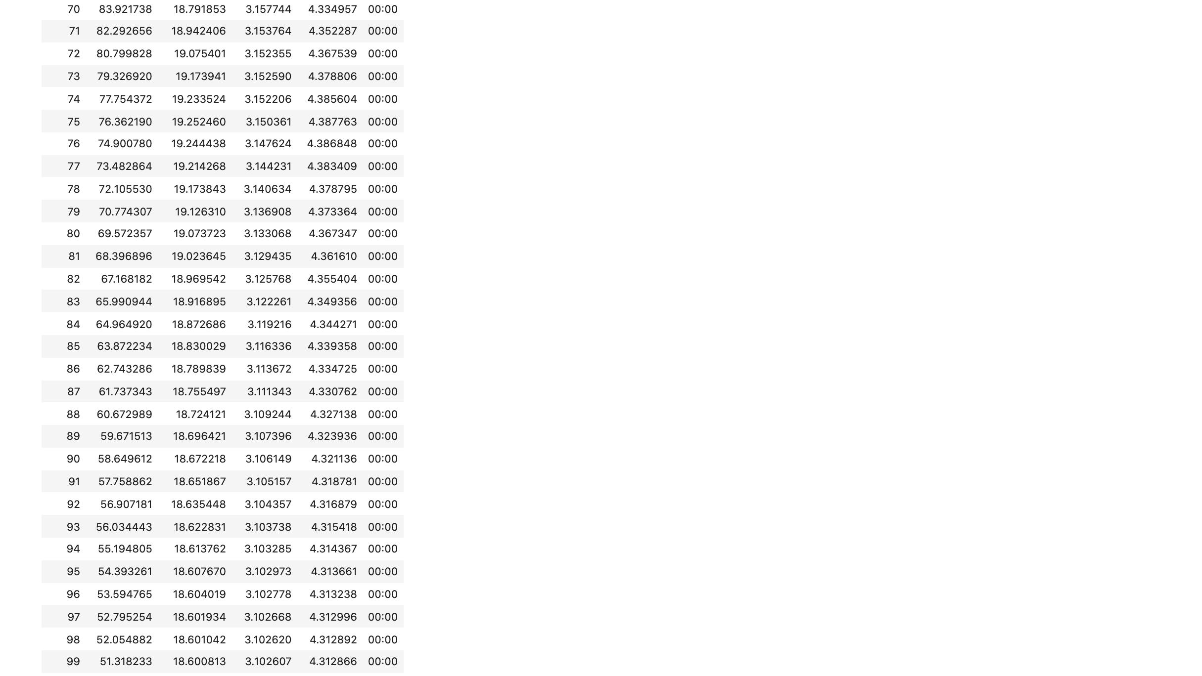
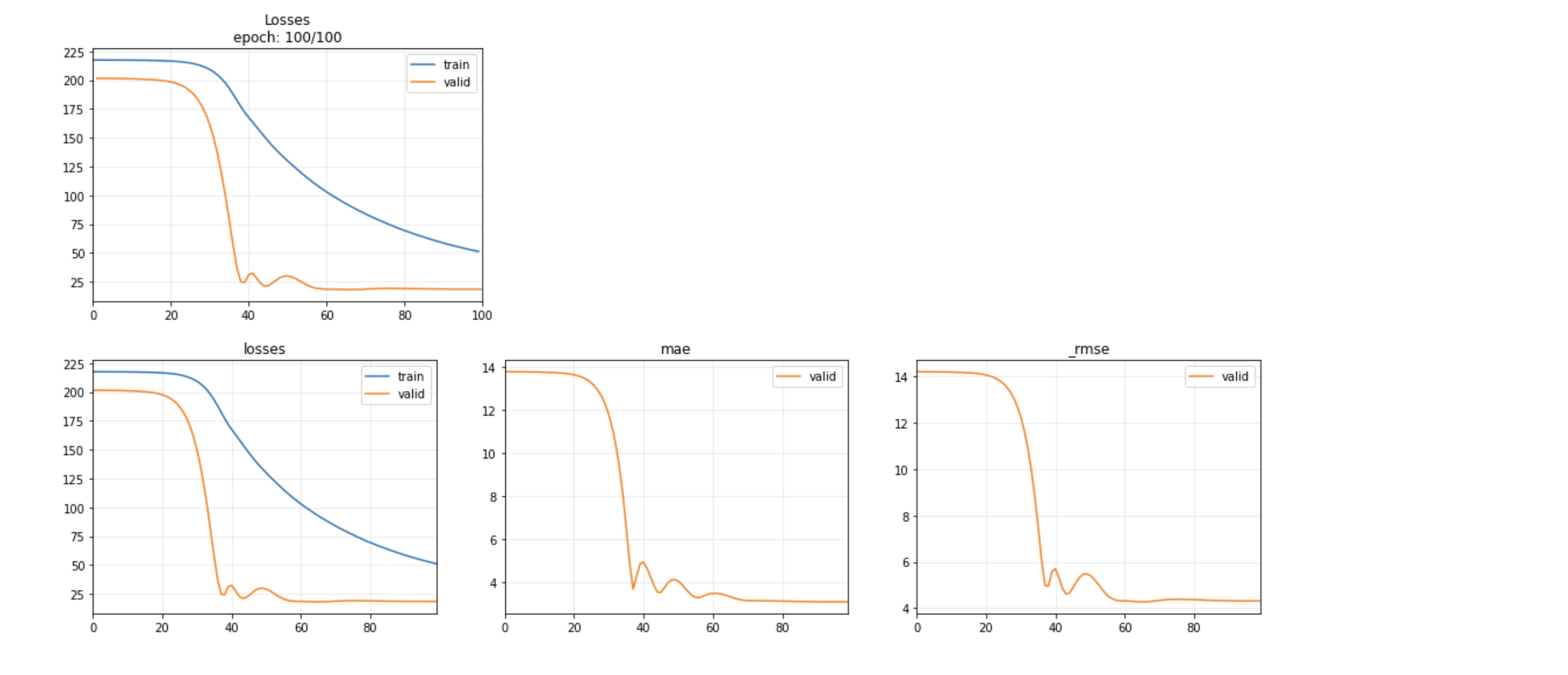
learn.fit_one_cycle(100, 8e-4)